RULE 2: COHESION (Avoid isolation)

In the last chapter, we discussed the first rule of Flocking: avoid overcrowding (separation). Now we are going to talk about the complement. Rule 2 roughly states that if you find yourself out on your own, move towards your neighbors. In the harsh reality of the predator-prey relationship, those that wander away or get separated from the group are the ones that are eaten. Follow Rule 2. It could save your life.

void ParticleController::applyForce( float zoneRadiusSqrd, float thresh )
    {
      for( list::iterator p1 = mParticles.begin(); p1 != mParticles.end(); ++p1 ) {
        list::iterator p2 = p1;
        for( ++p2; p2 != mParticles.end(); ++p2 ) {
          Vec3f dir = p1->mPos - p2->mPos;
          float distSqrd = dir.lengthSquared();

          if( distSqrd < zoneRadiusSqrd ) { // If the neighbor is within the zone radius...
            float percent = distSqrd/zoneRadiusSqrd;

            if( percent < thresh ) { // ... and is within the threshold limits, separate...
              float F = ( thresh/percent - 1.0f ) * 0.01f;
              dir = dir.normalized() * F;
              p1->mAcc += dir;
              p2->mAcc -= dir;
            }
            else { // ... else attract
              float threshDelta = 1.0f - thresh;
              float adjustedPercent = ( percent - thresh )/threshDelta;
              float F = ( 1.0 - ( cos( adjustedPercent * M_PI*2.0f ) * -0.5f + 0.5f ) ) * 0.04f;
              dir = dir.normalized() * F;
              p1->mAcc -= dir;
              p2->mAcc += dir;
            }
          }
        }
      }
    }

We still have the nested for-loop of list iterators from the last chapter. The thing that has changed is we now have an additional case for our distance (squared) checks. If the squared distance between two Particles is less than the threshold, then we want to repel. If the squared distance is greater, then we apply the attraction force.

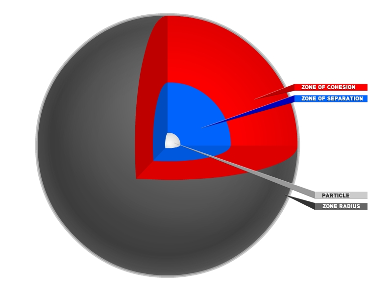
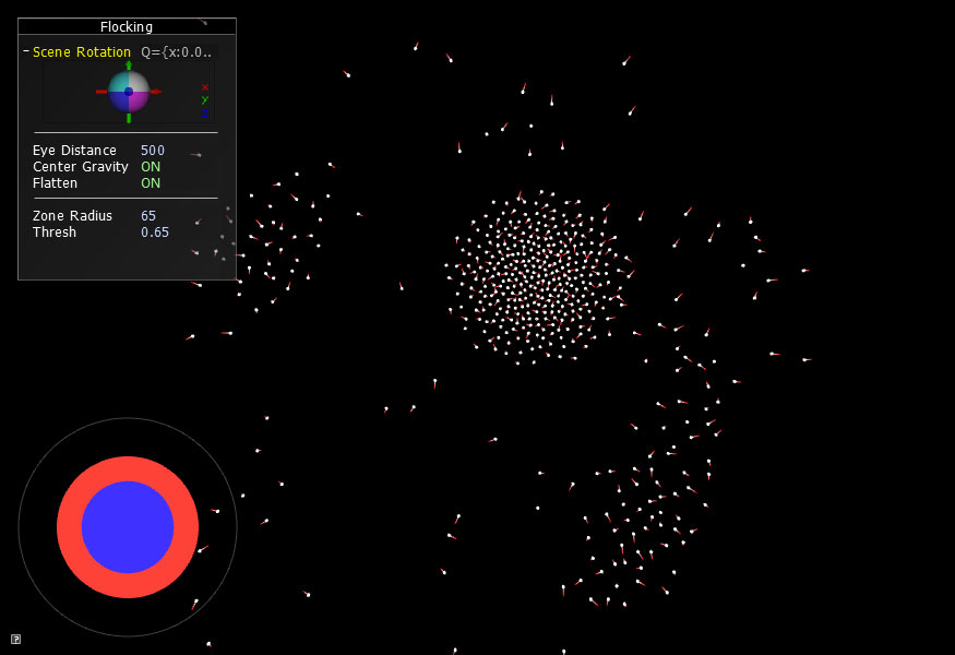
The reason we bother with this upper threshold limit (the zone radius) is two-fold. It is much more likely that flocking creatures pay attention to their nearest few neighbors as opposed to taking in the position of every single neighbor. In a flock of starlings, for example, it is theorized that each bird pays attention to 6 or 7 neighbors. Luckily for us, to only pay attention to a handful of neighbors eases the load on the processor. Sadly, we are still doing distance (squared) checks which we need for the threshold comparison, but at least we can rule out distant objects and not worry about the extra math in that if-else statement. (note: There are many ways to deal with this work load that would improve the performance dramatically, such as implementing a kd-tree or Octree. However, this will unnecessarily complicate the tutorial so we will leave that for a future chapter or as an exercise for the reader.)

I would like to draw attention to the Force variable again. It is without question the most confusing line in the applyForce() method.

If you look at the adjustedPercent variable, you should notice that it is normalizing the range that the percent variable can exist within. Basically, adjustedPercent is a variable that has a range from 0.0 to 1.0. Inside the cos(), we multiply our adjusted percentage by 2π so now we have a range from 0.0 to 2π.

Take a look at the picture below. The upper curve is what we have: cosine between 0.0 and 2π which creates a smooth undulation from 1.0 to -1.0 and back to 1.0. However, we want a curve we can use to control how much each particle attracts each other particle within the range. To do that, we need to turn the original curve into one that undulates from 0.0 to 1.0 and back to 0.0. All the Force equation is doing is finding a way to take our BEFORE curve and turn it into our AFTER curve.

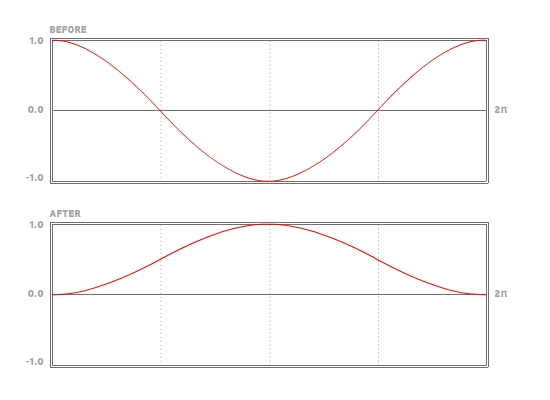
The reason we want to do this is so we can have a smooth transition as the neighbor particle goes from outside the range to inside the range. Otherwise, the particle movements through space would be more jarring and angular. We want smooth and blended movement. That is all the Force equation is doing.

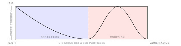
Think of it this way. The height of the black curve below shows the strength of the force at every position in the zone radius. The attractive force right on the very edge of the zone radius is zero, as it is right where the zone transitions from separation to cohesion.

As I mentioned in the last chapter, a large percentage of time is spent tweaking the F variable for the repulsion and attraction equations. If the attractive force is too strong, the flockers bunch up and resemble a swarm of gnats or flies. If the attractive force is too weak, the flockers barely seem to flock at all.

When you run the project, you will notice the difference between Chapter 2 and Chapter 3 isn't too pronounced. This is because we already added an attractive force in Chapter 1 in the form of the global gravitation towards the center of the screen. With the introduction of Particle-to-Particle attraction in this chapter, we don't really need that global gravitation as much as before. Since the Particles are pulling towards each other, they tend to want to hang out in a big group. If we turn off the gravity, the Particles will hover around the center of the screen for a while but will eventually wander and disappear from view.

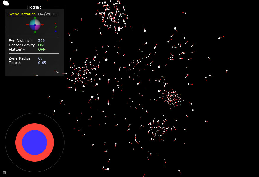
However, we did add a new boolean toggle called mFlatten. As you might imagine, turning on the flatten feature squashes the z-axis down to zero so you can better see how the Particles are pushing each other around. It is very useful for fine-tuning your force equations.

In Flocking Chapter 4, the third rule for the flocking system is explained. It is the rule of alignment which helps the particles behave as a group.